Showing posts with label chi-square. Show all posts

Tuesday, May 27, 2014

Chi-Square Independence Test in in 7 Steps in Excel 2010 and Excel 2013

Chi-Square Independence

Test in 7 Steps in Excel

The Chi-Square Independence Test is used to determine whether two categorical variables associated with the same item act independently on that item. The example presented in this section analyzes whether the gender of the purchaser of a car is independent of the color of the car. This Chi-Square Independence Test answers the question of whether gender plays a role in the color selection of a purchased car

Each item (each purchased car) has two attributes associated with it. These two attributes are the categorical variables of purchaser’s gender and color. The counts of the number of cars purchased for each unique combination of gender and color are placed in a matrix called a contingency table.

Contingency Table

A contingency table is a two-way cross-tabulation. Each row in the contingency table is associated with one of the levels of one of the categorical attributes (such as gender) and each column is associated with one of the levels of the other categorical attribute (such as color).

The number of rows in the contingency table, r, is equal to the number of levels of the row attribute. The number of columns in the contingency table, c, is equal to the number of levels of the column attribute. The contingency table is therefore an r x c table and has r x c cells representing r x c unique combinations of levels of row and column attributes.

Test Compares Actual vs.

Expected Bin Counts

The Chi-Square Independence Test compares whether counts of the actual data for each unique combination of factors of the two variables are significantly different than the counts that would be expected if the attributes were totally independent of each other.

Null Hypothesis

A Null Hypothesis is created which states there is no significant difference between the actual and expected counts of data for the unique combinations of levels of the two factors.

Test Statistic

The Chi-Square Independence Test calculates a Test Statistic called a Chi-Square Statistic, Χ². The distribution of this Test Statistic can be approximated by the Chi-Square distribution if several conditions are met.

When to Reject Null Hypothesis

The Null Hypothesis is rejected if that Chi-Square Statistic is larger than a Critical Chi-Square Value based upon the specified alpha level and degrees of freedom associated with that test. Equivalently, the Null Hypothesis is rejected if the p value derived from the test is smaller than the specified alpha level.

Required Assumptions

The distribution of this Test Statistic, Χ², can be approximated by the Chi-Square distribution with degrees of freedom equal to df = (r – 1)(c – 1) if the following three conditions are met:

1) The number of cells in the contingency table (r x c) is at least 5. A 2 x 2 contingency table is not large enough. One of the two attributes must have at least 3 levels.

2) The average value of all of the expected counts is at least 5.

3) All of the expected counts equal at least 1.

Example of Chi-Square

Independence Test in Excel

We will examine whether gender and product color selection are independent of each other. A car company in the United States sold new 12,000 cars of one brand in one month. The car company recorded the gender of each customer and also the color of the car. The car was available in only three colors: red, blue, and green. The actual counts of cars purchased in that months for each unique combination of gender/color are shown as follows:

Determine with 95-percent certainty the car purchaser’s gender and the selected color of the car are independent of each other.

Step 1 – Place Actual Counts In Contingency Table

The actual counts of the number of items having each unique combination of row and column attribute level are placed into the proper cell in the r x c contingency table. In this case the counts of the number of cars associated with each unique combination of gender/color are placed into the correct cells of the 2 x 3 contingency table as follows:

(Click Image To See Larger Version)

Creating the Contingency Table From an Excel Pivot Table

The contingency table can be created with Excel’s Pivot Table tool if the data are initially presented in the following fashion as they often are:

(Click Image To See Larger Version)

The Pivot Table is accessed from within the Insert tab.

Insert / Pivot Table / Pivot Table bring up the initial Pivot Table dialogue box. The table range and output location should be filled in as follows:

(Click Image To See Larger Version)

Hitting OK brings up the following final Pivot Table dialogue box:

(Click Image To See Larger Version)

Dragging the label Color down to the Column Labels box and to the Σ Values box and then dragging the label Gender down to the Row Labels box produces the completed Pivot Table as follows. This Pivot Table is an exact match of the contingency table containing the actual values for this data set.

(Click Image To See Larger Version)

Note that the Excel Pivot Table would be an exact match for the contingency table with the actual counts that is shown again here.

(Click Image To See Larger Version)

Step 2 – Place Expected Counts In Contingency Table

The expected counts for each unique combination of levels of row/column attributes are placed into the correct cells of an identical contingency table as follows:

(Click Image To See Larger Version)

The expected counts are based upon the assumption that the row and column attributed act independently of each other. The method of calculated the expected numbers based upon this assumption is shown below:

(Click Image To See Larger Version)

Step 3 – Create Null and Alternative Hypotheses

The Null Hypothesis states that there is no difference between the expected and actual counts of items for each unique combination of levels of row and column attributes. The Test Statistic, Χ², would equal 0 in this case. The Null Hypothesis is therefore specified as follows:

H₀: Χ² = 0

The Chi-Square Statistic, Χ², is distributed according to the Chi-Square distribution if the required assumptions for this tests that are specified in this blog article are met. The Chi-Square distribution has only one parameter: its degrees of freedom, df. The probability density function of the Chi-Square distribution calculated at x is defined as f(x,df) and can only be defined for positive values of x.

Since the Chi-Square’s PDF value f(x,df) only exists for positive values of x, the alternative hypothesis specifies that that the Chi-Square Independence Test is a one-tailed test in the right tail and is specified as follows:

H₁: Χ² > 0

Step 4 – Verify Required Assumptions

The distribution of this Test Statistic, Χ2, can be approximated by the Chi-Square distribution with degrees of freedom equal to df = (r – 1)(c – 1) if the following three conditions are met:

1) The number of cells in the contingency table (r x c) is at least 5. The contingency table is a 2 x 3 table so this condition is met.

2) The average value of all of the expected counts is at least 5. This condition is met.

3) All of the expected counts equal at least 1. This condition is met.

Step 5 – Calculate Chi-Square Statistic, Χ²

The Test Statistic, which is the Chi-Square Statistic, Χ², is calculated for n = r x c unique cells in the contingency table as follows:

(Click Image To See Larger Version)

This can be quickly implemented in a convenient table as follows: (Click Image To See Larger Version)

Step 6 – Calculate Critical Chi-Square Value and p Value

The degrees of freedom for the Chi-Square Independence Test is calculated as follows:

r = number of rows = 2

c = number of columns = 3

df = (r – 1)(c – 1) = (2 – 1)(3 – 1) = 2

The Critical Chi-Square Value is calculated as follows:

Chi-Square Critical = CHISQ.INV.RT(α,df)

Chi-Square Critical = CHISQ.INV.RT(0.05,2) = 5.99

Prior to Excel 2010, the formula is calculated as follows:

Chi-Square Critical = CHIINV(α,df)

The p Value is calculated as follows:

p Value = CHISQ.DIST.RT(Chi-Square Statistic,df)

p Value = CHISQ.DIST.RT(6.17,2) = 0.0457

Prior to Excel 2010, the formula is calculated as follows:

p Value = CHIDIST(Chi-Square Statistic,df)

Step 7 – Determine Whether To Reject Null Hypothesis

The Null Hypothesis is rejected if either of the two equivalent conditions are shown to exist:

1) Chi-Square Statistic > Critical Chi-Square Value

2) p Value < α

Both of these conditions exist as follows.

Chi-Square Statistic = 6.17

Critical Chi-Square value = 5.99

p Value = 0.0457

α = 0.05

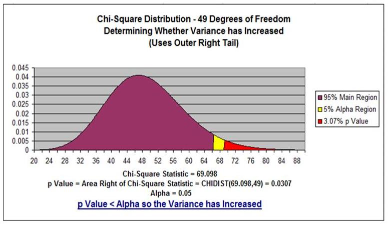
In this case we reject the Null Hypothesis because the Chi-Square Statistic (6.17) is larger than the Critical Value (5.99) or, equivalently, the p Value (0.0457) is smaller than Alpha (0.05). A graphical representation of this problem is shown as follows in this Excel-generated graph:

(Click Image To See Larger Version)

Excel Master Series Blog Directory

Statistical Topics and Articles In Each Topic

Technorati Tags: excel,excel 2010,excel 2013,statistics,chi-square,chi-square independence test,chi square,chi square independence test,hypothesis test,contingency table

Saturday, May 22, 2010

How To Find Out if Your Customers are Becoming More or Less Predictable in Their Spending With the Chi-Square Variance Test in Excel

Chi-Square Population

Variance Test in Excel

for Marketing

It’s hard to predict exactly how much each one of your new customers will buy, but you probably have a good idea of the range that you would expect your customer’s spending to fall within.

What if you suddenly noticed a blip in recent customer order amounts which indicated that your customer spending spread might be widening? Is there a way know for sure whether the spending spread really has widened, or is this just a temporary aberration that grabbed your attention but may not mean anything?

In statistical terms, the question you would be asking is: Has the standard deviation of my customers’ order size increased? Good news --> There is a convenient statistical test you can quickly run in Excel to find that out. The test is called the Chi-Square Variance Test and is used to determine if the variance of a population has changed. Variance equals the standard deviation squared so if a population’s standard deviation increases, so does its variance, to an even greater degree.

The Chi-Square Variance Test is a great and simple way to determine whether your customers are more or less focused in their purchases of you products. More importantly, the Chi-Square Variance Test tells you whether your customers are being affected by something is changing what they buy from your company.

If variance of your customers’ spending has become smaller, your customer order size has become more predictable and more focused. If the variance has increased, your customer order size has become less predictable and less focused.

This Test Will Not Tell You What Changed, Only That Something Has Changed.

If the range (standard deviation) of customer spending on individual orders changes, the product mix that your customers normally purchase is changing. The underlying reason for this probably has important implications for the marketing program. If standard deviation (and therefore the variance) of order size changes, you will want to investigate further and find out why.

Here is a video that will demonstrate step-by-step how to perform the Chi-Square Variance Test in Excel to determine if the majority of your customers really have become more or less focused in their spending on individual orders.

Here is a Step-By-Step Video Showing How to Find Out If Your Customers Have Become More or Less Focused In Their Spending By Using the Chi-Square Variance Test in Excel:

(Is Your Sound Turned On?)

What Is the Chi-Square Variance Test?

The Chi-Square Variance Test and is used to determine if the variance of a population has changed. Marketers use the Chi-Square Variance Test to determine if the expected range of customer spending is changing. If so, something is affecting the buying habits of the customers.

The Chi-Square Variance Test consists of just 2 calculations that require only 4 inputs total.

These 4 inputs are:

1) Historic Standard Deviation, σ, of the population – This would be the long-time standard deviation of customer spending per order. It shouldn’t be too hard to calculate a standard deviation of past customer order size. Population Standard Deviation is usually denoted as σ, sigma.

2) Standard Deviation, s, of a recent large (at least 30) sample drawn randomly from the population. Make sure that the sample is random and is representative of the population from which the Population Standard Deviation was taken. Sample Standard Deviation is usually denoted as s.

3) The Sample Size, n.

4) The Degree of Certainty desired in the test. For example, you might want to be at least 95% certain of the outcome determined by the test.

The Chi-Square Variance Test requires measurements of standard deviation, not variance. That has no effect because, as mentioned above, variance is derived from standard deviation. Variance equals standard deviation squared.

The 5 Steps of the Chi-Square Variance Test

There are 5 steps in the Chi-Square Variance Test. They are;

Step 1) Determine the Required Level of Certainty, and, therefore, α, Alpha.

Step 2) Measure Sample Standard Deviation (s) from a large recent random sample drawn from the same population from which the Population Standard Deviation (σ) was derived. Sample size, n, must be at least 30.

Step 3) Calculate the Chi-Square Statistic.

Chi-Square Statistic = [ (n-1)*(s*s) ] / [σ*σ]

Step 4) Calculate the Curve Area Outside of the Chi-Square Statistic.

There are 2 possibilities:

a) If Sample Standard Deviation, s, is greater than the population Standard Deviation (σ):

Calculate the Area in the Right Outer Tail to the Right of the Chi-Square Statistic by this formula:

Tail Area Right of Chi-Square Statistic =
CHIDIST( Chi-Square Statistic, n-1 )

In this blog article and attached video, we will color the tail area outside the chi-Square Statistic with RED.

We will also color the area under the curve that represents alpha with yellow, as follows:

The 5% Alpha Area (Yellow) Resulting
From 95% Required Certainty

chi squared in excel, chi square, anova, chi square test, chi square distribution, statistical analysis in excel

Click on the Image To See a Larger Version

The Red Area Outside the Chi-Square Statistic
(Is Smaller Than the Yellow Alpha Area)

Click on the Image To See a Larger Version

b) If Sample Standard Deviation, s, is less than the population Standard Deviation, σ,

then: Calculate the Area in the Left Outer Tail to the Left of the Chi-Square Statistic Tail:

Tail Area Left of Chi-Square Statistic =
1 - CHIDIST( Chi Square Statistic, n-1 )

The 5% Alpha Area (Yellow) Resulting
From the 95% Required Certainty

Click on the Image To See a Larger Version

The Red Area Outside the Chi-Square Statistic
(Is Larger Than the Yellow Alpha Area)

Click on the Image To See a Larger Version

The area under the Chi-Square curve that lies outside of the Chi-Square Statistic is sometimes called the P Value. For example, if 3% of the curve area lies outside the Chi-Square Statistic, then the P Value is 0.03.

Step 5) Analyze Using the Chi-Square Statistic Rule: If the area under the curve outside the Chi-Square Statistic is less than alpha, the population variance has moved in the direction of Sample Standard Deviation.

For example, if alpha is 0.05 (you require 95% certainty and alpha is therefore 0.05) and only 3% of the area under the Chi-Square curve lies outside of the Chi-Square Statistic, then you can now state with 95% certainty that the variance had moved.

The variance would have moved in the direction of the Sample Standard Deviation. If Sample Standard Deviation was measured to be greater the Population Standard Deviation and the curve area outside of the Chi-Square Statistic (3% = 0.03) was less than alpha (0.05), you can state with 95% certainty that population variance has increased.

To sum it up with charts:

If the red area fits inside the yellow area, we can state with the required degree of certainty that the population variance has moved in the direction of the sample standard deviation. In the case directly below, the red area does fit inside the yellow (alpha) area so we can state that the population varianced moved to the right (increased), with 95% certainty:

The Red Area Outside the Chi-Square Statistic
Is Smaller Than the Yellow Alpha Area

Click on the Image To See a Larger Version

If the red area DOES NOT fit inside the yellow area, we CANNOT state with the required degree of certainty that the population variance has moved in the direction of the sample standard deviation. In the case directly below, the red area DOES NOT fit inside the yellow (alpha) area so we CANNOT state that the population varianced moved to the left (decreased), with 95% certainty:

The Red Area Outside the Chi-Square Statistic
Is Larger Than the Yellow Alpha Area

Click on the Image To See a Larger Version

Here is the Test We Ran

Here is the problem definition: Customers on a commercial web site have historically had a standard deviation of 1.6 in the number of items they buy on individual purchase orders. The company’s Internet marketing manager took a random sample of 50 recent orders and measured the standard deviation of that sample to be 1.9 items per order.

The Internet marketing manager wanted to know with at least 95% certainty whether the population standard deviation had increased (had moved in the direction of the sample standard deviation).

The Required 4 Pieces of Information

1) Population Standard Deviation, σ, of item per order = 1.6

2) Sample Standard Deviation, s, of items per order = 1.9

3) Sample size, n = 50

4) Required Level of Certainty = 95%

The 5 Steps of the Chi-Square Variance Test

Using the 5-Step Chi-Square Variance Process, the Internet Marketing Manager determines within 95% certainty whether the population variance has increased as follows.

Step 1) Determine the Required Level of Certainty, and, therefore α, Alpha.

The Required Level of Certainty is 95%. Alpha, α, is 0.05.

Alpha = 1 – Required Level of Certainty = 1 – 95% = 0.05

Step 2) Measure Sample Standard Deviation (s) from a recent, large, representative random sample drawn from the same population from which the Population Standard Deviation (σ) was derived.Sample Standard Deviation, s, of items per order = 1.6. Population Standard Deviation, σ, of item per order = 1.6

Step 3) Calculate the Chi-Square StatisticChi-Square Statistic = [ (n-1)*(s*s) ] / [σ*σ]Chi-Square Statistic = [ (50 - 1) * (1.9 * 1.9) ] / [1.6 * 1.6] = 69.09766

Step 4) Calculate the Curve Area Outside of the Chi-Square Statistic

If Sample Standard Deviation, s, is greater than the population Standard Deviation (σ):

then calculate the Area in the Right Outer Tail outside of the Chi-Square Statistic by this formula:

Tail Area Right of Chi-Square Statistic =

CHIDIST( Chi-Square Statistic, n-1 )

Since s is greater than σ,

Tail Area Right of Chi-Square Statistic =
CHIDIST( Chi-Square Statistic, n-1 )

Tail Area Right of Chi-Square Statistic =

CHIDIST( 69.09766, 49 ) = 3.07

So area under the curve outside the Chi-Square Statistic = 3.07%

The P Value = 0.0307

The Red Area Outside the Chi-Square Statistic
(Is Smaller Than Alpha) in the Outer Right Tail
So We Can State With 95% Certainty That
the Population Variance Have Moved to the
Right (Increased)

Click on the Image To See a Larger Version

Step 5) Analyze Using the Chi-Square Statistic Rule: If the P Value (P Value = 0.0307), the area under the curve outside the Chi-Square Statistic, is less than α (α = 0.05), the population variance has moved in the direction of Sample Standard Deviation.

We can see that the red area fits inside of the yellow area on the outer right tail. In this case, the area outside the Chi-Statistic (3.07%) is less than Alpha (5%), we can state with 95% certainty that the population variance has increased.

Now the Internet marketing manager needs to determine the underlying reason why customer spending has become less focused.

Conclusion - The Chi-Square Variance Test Tells Whether Something Has Changed Your Customers' Buying Habits

Incidentally, all of the Chi-Square Probability Density Function graphs in this article had 49 Degrees of Freedom. Degrees of Freedom is derived from sample size and equals n-1 (50 - 1 = 49 Degrees of Freedom).

Here are links to other training videos of how to create interactive graphs in Excel of some of the other major statistical distributions:
How to Graph the Normal Distribution's Probability Density Function in Excel

How To Graph the Normal Distribution's Cumulative Distribution Function in Excel

How To Graph the Students t Distributions' Probability Density Function in Excel

How To Graph the Chi-Square Distribution's Probability Density Function in Excel

How To Graph the Weibull Distribution's PDF and CDF - in Excel

If you have any questions or comments about this article and attached videos, please post them below. Your opinion is highly valued

Excel Master Series Blog Directory

Statistical Topics and Articles In Each Topic

Subscribe to: Posts (Atom)

Become an Excel Statistical Master

Excel Master Series - MBA-level statistics - Over 1,100+ Pages of Easy-To-Follow Instructions in Excel

It's a Full
Easy-To-Follow
MBA Course in Business Statistics

ALL IN EXCEL

&

MUCH Clearer

Than Your Text

Book

Download the
1,100+ Page Excel Statistical Master now

More Easy-To-

Follow eManuals

That You Will

Master Quickly

Step-By-Step Optimization With Excel Solver

What's In It?

For anyone who wants to be operating at a high level with the Excel Solver quickly, this is the book for you. Step-By-Step Optimization With Excel Solver is a 200+ page .pdf e-manual of simple yet thorough explanations on how to use the Excel Solver to solve today’s most widely known optimization problems. Loaded with screen shots that are coupled with easy-to-follow instructions, this book will simplify many difficult optimization problems and make you a master of the Excel Solver almost immediately.

Here are just some of the Solver optimization problems that are solved completely with simple-to-understand instructions and screen shots in this e-manual:

• The famous “Traveling Salesman” problem using Solver’s Alldifferent constraint and the Solver’s Evolutionary method to find the shortest path to reach all customers. This also provides an advanced use of the Excel INDEX function.

• The well-known “Knapsack Problem” which shows how optimize the use of limited space while satisfying numerous other criteria.

• How to perform nonlinear regression and curve-fitting on the Solver using the Solver’s GRG Nonlinear solving method.

• How to solve the “Cutting Stock Problem” faced by many manufacturing companies who are trying to determine the optimal way to cut sheets of material to minimize waste while satisfying customer orders.

• Portfolio optimization to maximize return or minimize risk.

• Venture capital investment selection using the Solver’s Binary constraint to maximize Net Present Value of selected cash flows at year 0. Clever use of the If-Then-Else statements makes this a simple problem.

• How use Solver to minimize the total cost of purchasing and shipping goods from multiple suppliers to multiple locations.

• How to optimize the selection of different production machine to minimize cost while fulfilling an order.

• How to optimally allocate a marketing budget to generate the greatest reach and frequency or number of inbound leads at the lowest cost.

Step-By-Step Optimization With Excel Solver has complete instructions and numerous tips on every aspect of operating the Excel Solver. You’ll fully understand the reports and know exactly how to tweek all of the Solver’s settings for total custom use. This e-manual also provides lots of inside advice and guidance on setting up the model in Excel so that it will be as simple and intuitive as possible to work with.

All of the optimization problems in this book are solved step-by-step using a 6-step process that works every time. In addition to detailed screen shots and easy-to-follow explanations on how to solve every optimization problem in the book, a link is provided to download an Excel workbook that has all problems completed exactly as they are in this e-manual.

Step-By-Step Optimization With Excel Solver is exactly the e-manual you need if you want to be optimizing at an advanced level with the Excel Solver quickly.

*******************

Become an Excel Statistical Master

It's a Full
Easy-To-Follow
MBA Course in Business Statistics

ALL IN EXCEL

&

MUCH Clearer

Than Your Text

Book

Download the
1,100+ Page Excel Statistical Master now

More Easy-To-

Follow eManuals

That You Will

Master Quickly

*******************

Become an Excel Statistical Master

It's a Full
Easy-To-Follow
MBA Course in Business Statistics

ALL IN EXCEL

&

MUCH Clearer

Than Your Text

Book

Download the
1,100+ Page Excel Statistical Master now

More Easy-To-

Follow eManuals

That You Will

Master Quickly

*******************

Become an Excel Statistical Master

It's a Full
Easy-To-Follow
MBA Course in Business Statistics

ALL IN EXCEL

&

MUCH Clearer

Than Your Text

Book

Download the
1,100+ Page Excel Statistical Master now

Immediate, Absolute, No-Questions-Asked, Money-Back Guarantee If Not TOTALLY, 100% Satisfied. In Other Words, If Any Excel Master Series eManual That You've Purchased Here Does Not Provide Instructions That Are CRYSTAL CLEAR and EASY TO UNDERSTAND, You Get All Of Your Money Back Immediately and Keep the eManual. Guaranteed!

Meet The Author